Polimini e grafi
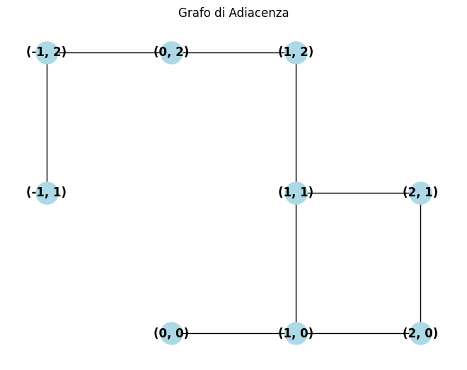
A un polimino possiamo associare il grafo, quello delle adiacenze, che ha per nodi le sue celle e per archi i lati che le celle hanno in comune. NetworkX è un pacchetto Python per la creazione, la manipolazione e lo studio della struttura, della dinamica e delle funzioni di reti complesse.
import networkx as nx
def adjacency_graph(S):
G = nx.Graph()
# Aggiungi archi tra quadrati adiacenti
lst_S = list(S)
for i, (xi, yi) in enumerate(lst_S):
for j, (xj, yj) in enumerate(lst_S[i+1:], i+1):
# Controlla adiacenza (differenza di 1 in una coordinata e uguale nell'altra)
if ((abs(xi - xj) == 1 and yi == yj) or (abs(yi - yj) == 1 and xi == xj)):
G.add_edge((xi, yi), (xj, yj))
return G
S = {(0,0), (1,0), (2,0), (2,1), (1,1), (1,2), (0,2), (-1,2), (-1,1)}
nx.draw(adjacency_graph(S), {s: s for s in S},
with_labels=True, node_color='lightblue',
node_size=500, font_weight='bold')
plt.title("Grafo di Adiacenza")
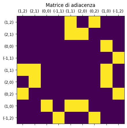
La matrice di adiacenza è qualcosa di analogo: a righe e colonne sono associate le celle, troviamo 1 o 0 in una certa riga e a una certa colonna se le due celle rappresentate sono adiacenti oppure no.
def adjacency_matrix(S):
n = len(S)
matrix = [[0] * n for _ in range(n)]
lst_S = list(S)
for i, (xi, yi) in enumerate(lst_S):
for j, (xj, yj) in enumerate(lst_S[i+1:], i+1):
if ((abs(xi - xj) == 1 and yi == yj) or
(abs(yi - yj) == 1 and xi == xj)):
matrix[i][j] = 1
matrix[j][i] = 1
return matrix
print("Matrice di adiacenza:")
for row in adjacency_matrix(S):
print(row)
Matrice di adiacenza:
[0, 0, 0, 0, 1, 0, 1, 0, 0]
[0, 0, 0, 0, 1, 1, 0, 0, 0]
[0, 0, 0, 0, 0, 0, 0, 1, 0]
[0, 0, 0, 0, 0, 0, 0, 0, 1]
[1, 1, 0, 0, 0, 0, 0, 1, 0]
[0, 1, 0, 0, 0, 0, 0, 1, 0]
[1, 0, 0, 0, 0, 0, 0, 0, 1]
[0, 0, 1, 0, 1, 1, 0, 0, 0]
[0, 0, 0, 1, 0, 0, 1, 0, 0]
matrice che può essere rappresentata graficamente.
plt.matshow(adjacency_matrix(S))
plt.xticks(ticks=np.arange(len(S)), labels=[f"({x},{y})" for x,y in list(S)])
plt.yticks(ticks=np.arange(len(S)), labels=[f"({x},{y})" for x,y in list(S)])
plt.title("Matrice di adiacenza")
plt.show()
In particolare potremmo individuare il cammino più breve usando il metodo .shortest_path().
nx.shortest_path(G, source=(0,0), target=(-1,2))
[(0, 0), (1, 0), (1, 1), (1, 2), (0, 2), (-1, 2)]
Un'articolata analisi del grafo può essere fatta come di seguito.
def analyze_connectivity(S):
G = adjacency_graph(S)
properties = {
'number_of_squares': len(S),
'diameter': nx.diameter(G) if nx.is_connected(G) else float('inf'),
'average_shortest_path': nx.average_shortest_path_length(G),
'connectivity': nx.node_connectivity(G),
'articulation_points': list(nx.articulation_points(G)),
'biconnected_components': list(nx.biconnected_components(G)),
'is_biconnected': nx.is_biconnected(G),
'degree_sequence': [d for n, d in G.degree()],
'is_tree': nx.is_tree(G)
}
return properties
properties = analyze_properties(S)
for key, value in properties.items():
print(f"{key}: {value}")
number_of_squares: 9
diameter: 6
average_shortest_path: 2.7777777777777777
connectivity: 1
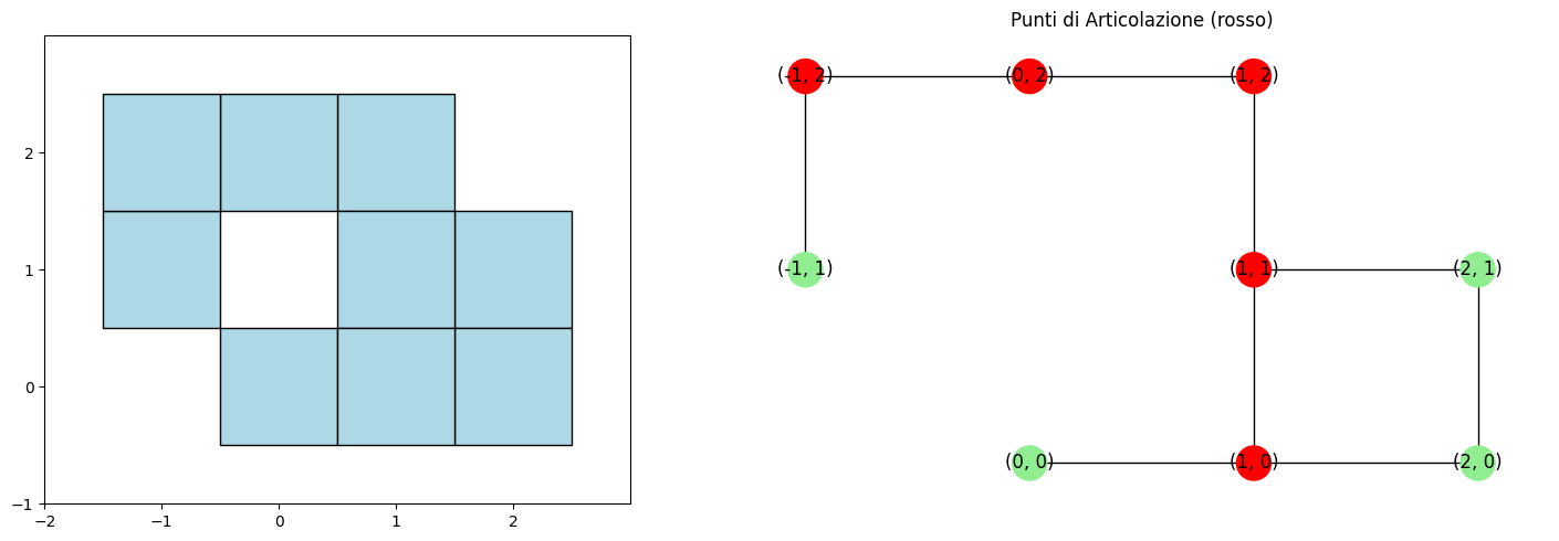
articulation_points: [(1, 0), (1, 1), (-1, 2), (0, 2), (1, 2)]
biconnected_components: [{(1, 0), (0, 0)}, {(1, 0), (1, 1), (2, 0), (2, 1)}, {(1, 1), (1, 2)}, {(-1, 1), (-1, 2)}, {(0, 2), (-1, 2)}, {(0, 2), (1, 2)}]
is_biconnected: False
degree_sequence: [2, 3, 2, 2, 2, 1, 3, 1, 2]
is_tree: False
Una rappresentazione grafica completa dell'insieme e del grafo delle adiacenze con i punti di articolazione.
def plot_analysis(S):
fig, axes = plt.subplots(1, 2, figsize=(15, 5))
# 1. Visualizzazione del polimino
axes[0].set_aspect('equal')
for (x, y) in S:
axes[0].add_patch(plt.Rectangle((x-0.5, y-0.5), 1, 1,
facecolor='lightblue',
edgecolor='black'))
axes[0].set_xlim(min(x for (x, y) in S)-1, max(x for (x, y) in S)+1)
axes[0].set_ylim(min(y for (x, y) in S)-1, max(y for (x, y) in S)+1)
axes[0].set_xticks(range(min(x for x,_ in S)-1, max(x for x,_y in S)+1))
axes[0].set_yticks(range(min(y for _,y in S)-1, max(y for _,y in S)+1))
# 2. Analisi di connettività
G = adjacency_graph(S)
pos = {s: s for s in S}
analysis = analyze_connectivity(S)
node_colors = ['red' if node in analysis['articulation_points']
else 'lightgreen' for node in G.nodes()]
nx.draw(G, pos, ax=axes[1], node_color=node_colors,
with_labels=True, node_size=500)
axes[1].set_title('Punti di Articolazione (rosso)')
plt.tight_layout()
plt.show()
G = adjacency_graph(S)
nx.shortest_path_length(G, source=(0,0), target=(-1,2))
5
Potrebbe essere utile un grafo che ha per archi, anziché i lati comuni alle celle, i vertici comuni.
def vert_graph(S):
G = nx.Graph()
# Aggiungi archi tra quadrati adiacenti
lst_S = list(S)
for i, (xi, yi) in enumerate(lst_S):
for j, (xj, yj) in enumerate(lst_S[i+1:], i+1):
# Controlla adiacenza (differenza di 1 in una coordinata e uguale nell'altra)
if ((abs(xi - xj) == 1 and yi == yj) or (abs(yi - yj) == 1 and xi == xj)):
G.add_edge((xi, yi), (xj, yj), weight=2)
if abs(xi - xj) == 1 and abs(yi - yj) == 1 :
G.add_edge((xi, yi), (xj, yj), weight=1)
return G
G = vert_graph(S)
nx.draw(G, {s: s for s in S},
with_labels=True, node_color='lightblue',
node_size=500, font_weight='bold')
nx.draw_networkx_edge_labels(G, {s: s for s in S},
edge_labels=nx.get_edge_attributes(G, 'weight'),
font_size=10)
plt.title("Grafo dei vertici comuni")
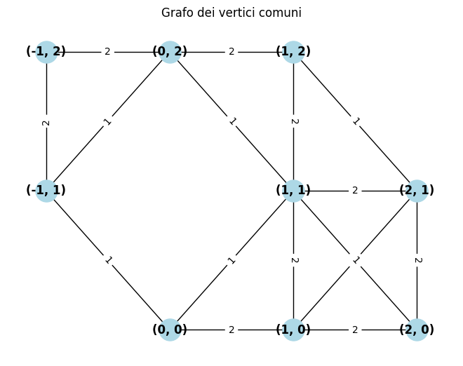
Il sottografo con gli stessi nodi e per archi solo quelli con peso 2 è il grafo delle adiacenze.