Seleziona alcune celle della seguente griglia quadrata $N\times N$ con
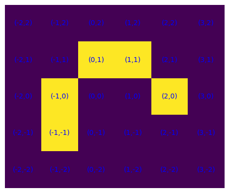
Possiamo rappresentare una cella di un reticolo quadrato con coordinate intere e quindi, in Python, un insieme di celle possiamo rappresentarlo con la struttura dati set come
S = {(-1,0),(-1,-1),(0,1),(1,1),(2,0)}
Per rappresentare graficamente l'insieme possiamo ad esempio vedere la griglia come una matrice di 0 e 1 e quindi visualizzarla con il metodo .matshow() della libreria matplotlib.
import matplotlib.pyplot as plt
def plot_S(S, coord=True):
x_S = [x for x,_ in S]
y_S = [y for _,y in S]
min_x = min(x_S)
max_y = max(y_S)
matrice = np.zeros((max_y-min(y_S)+3, max(x_S)-min_x+3))
for (x,y) in S:
matrice[max_y-y+1, x-min_x+1] = 1
plt.matshow(matrice)
plt.axis('off')
if coord:
for i in range(len(matrice)):
for j in range(len(matrice[0])):
plt.text(j, i, f"({j+min_x-1},{max_y-i+1})",ha="center", va="center", color="b")
plt.show()
plot_S(S)
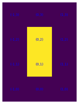
Possiamo associare a un insieme di celle S il sottinsieme di quelle "interne" nel modo seguente.
def interno(S):
I = set()
for (x,y) in S:
if len({(x+1,y), (x,y+1), (x-1,y),(x,y-1)} & S)==4:
I.add((x,y))
return I
L'insieme delle celle di S non interne ad esso, che hanno lati perimetrali, possiamo anche chiamarlo "bordo (o frontiera o limite o confine) interno".Possiamo anche considerare le celle non di S ma intorno a S, che potremmo chiamare "bordo (o frontiera o limite o confine) esterno", quelle nelle quali sarebbe possibile fare "scivolare" celle del bordo interno di S.
def bordoEst(S):
B = set()
for (x,y) in S:
B = B | {(x+1,y), (x,y+1), (x-1,y),(x,y-1)}-S
return B
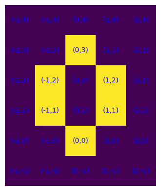
S = {(-1,2), (-1,1), (0,1), (0,2), (0,0), (1,1), (1,2), (0,3)}
plot_S(S), plot_S(interno(S)), plot_S(S-interno(S)), plot_S(bordoEst(S))
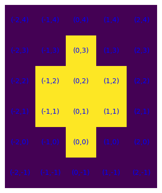
Per una rappresentazione non distinta delle diverse parti di S o correlate ad esso ci si può affidare a una procedura di visualizzazione, sempre mediante matrice, così modificata.
def plot_S(*Ss, coord=True):
min_x, min_y = np.inf, np.inf
max_x, max_y = -np.inf, -np.inf
for S in Ss:
if S:
x_m, x_M = min([x for x,_ in S]), max([x for x,_ in S])
y_m, y_M = min([y for _,y in S]), max([y for _,y in S])
min_x = x_m if x_m < min_x else min_x
min_y = y_m if y_m < min_y else min_y
max_y = y_M if y_M > max_y else max_y
max_x = x_M if x_M > max_x else max_x
matrice = np.zeros((max_y-min_y+3, max_x-min_x+3))
for i,S in enumerate(Ss):
for (x,y) in S:
matrice[max_y-y+1, x-min_x+1] = (len(Ss)-i)*10
plt.matshow(matrice)
plt.axis('off')
if len(S) < 50 and coord:
for i in range(len(matrice)):
for j in range(len(matrice[0])):
plt.text(j, i, f"({j+min_x-1},{max_y-i+1})",ha="center", va="center", color="b")
plt.show()
S = {(-1,2), (-1,1), (0,1), (0,2), (0,0), (1,1), (1,2), (0,3)}
plot_S(S,interno(S),S-interno(S),bordoEst(S))

Possiamo anche operare sugli insiemi di celle mediante traslazioni, simmetrie rispetto a una cella o rispetto ad assi, formati da celle, paralleli a quelli coordinati.
def trasOP(S,OP):
lstx, lsty = zip(*S)
x_OP, y_OP = OP
lstx, lsty = [x+x_OP for x in lstx], [y+y_OP for y in lsty]
return set(zip(lstx,lsty))
def simmC(S,C):
lstx, lsty = zip(*S)
x_C, y_C = C
lstx, lsty = [2*x_C-x for x in lstx], [2*y_C-y for y in lsty]
return set(zip(lstx,lsty))
def simmAss(S,asse,C):
lstx, lsty = zip(*S)
x_C, y_C = C
if asse == 'y':
lstx = [2*x_C-x for x in lstx]
else:
lsty = [2*y_C-y for y in lsty]
return set(zip(lstx, lsty))
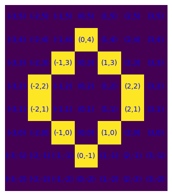
S = {(-1,0),(-1,-1),(0,1),(1,1),(2,0),(-2,-1)}
plot_S(S,simmC(S,(0,1)), S & simmC(S,(0,1)))
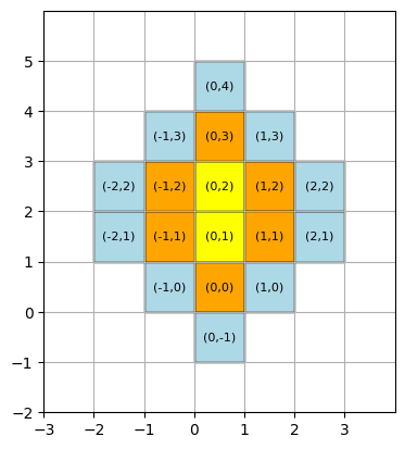
Per rappresentare graficamente le celle di una griglia quadrata si può usare anche altri metodi della libreria matplotlib.
def plot_R(*Ss, colors=['yellow','orange','red','green','blue']):
min_x, min_y = np.inf, np.inf
max_x, max_y = -np.inf, -np.inf
for S in Ss:
if S:
x_m, x_M = min([x for x,_ in S]), max([x for x,_ in S])
y_m, y_M = min([y for _,y in S]), max([y for _,y in S])
min_x = x_m if x_m < min_x else min_x
min_y = y_m if y_m < min_y else min_y
max_y = y_M if y_M > max_y else max_y
max_x = x_M if x_M > max_x else max_x
fig, ax = plt.subplots()
ax.set_aspect('equal')
for i,S in enumerate(Ss):
for (x, y) in S:
ax.add_patch(plt.Rectangle((x, y), 1, 1,
facecolor=colors[i],
edgecolor='black'))
ax.text(x+0.5, y+0.5, f'({x},{y})', ha='center', va='center', fontsize=8)
# Impostazione range assi
ax.set_xlim(min_x-1, max_x+2)
ax.set_ylim(min_y-1, max_y+2)
# Impostazione tick interi per entrambi gli assi
ax.set_xticks(range(min_x-1, max_x+2))
ax.set_yticks(range(min_y-1, max_y+2))
ax.grid(True)
plt.show()
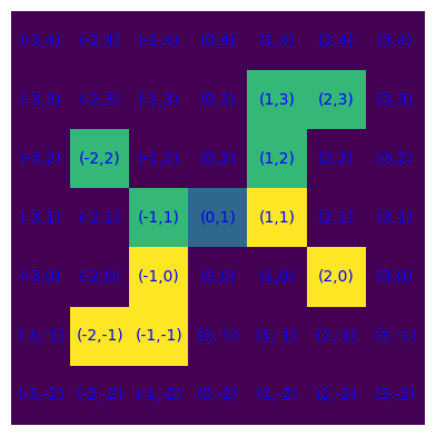
S = {(-1,2), (-1,1), (0,1), (0,2), (0,0), (1,1), (1,2), (0,3)}
plot_R(interno(S),S-interno(S),bordoEst(S),colors=['yellow','orange','lightblue'])